Integrating Foundational Time Series Models with PyMC-Marketing MMM

This tutorial demonstrates how to combine Chronos-2, a pretrained time series forecasting model, with PyMC-Marketing Media Mix Models (MMM). The goal is to forecast sales when control variables are unavailable for future periods.

This tutorial is based on the original notebook by Luca Fiaschi.

The Problem

When using MMM for forward-looking predictions, practitioners face a common challenge: control variables are often unavailable for future periods. Consider a scenario where your MMM includes employment rates and temperature as controls. These variables help the model separate media effects from external factors, but when planning next quarter’s media budget, you don’t yet have next quarter’s employment or temperature data.

This creates a practical dilemma:

• Without controls: Predictions may be biased because the model expects control inputs

• With naive assumptions (e.g., using last known values): Predictions degrade as the forecast horizon extends

The Approach

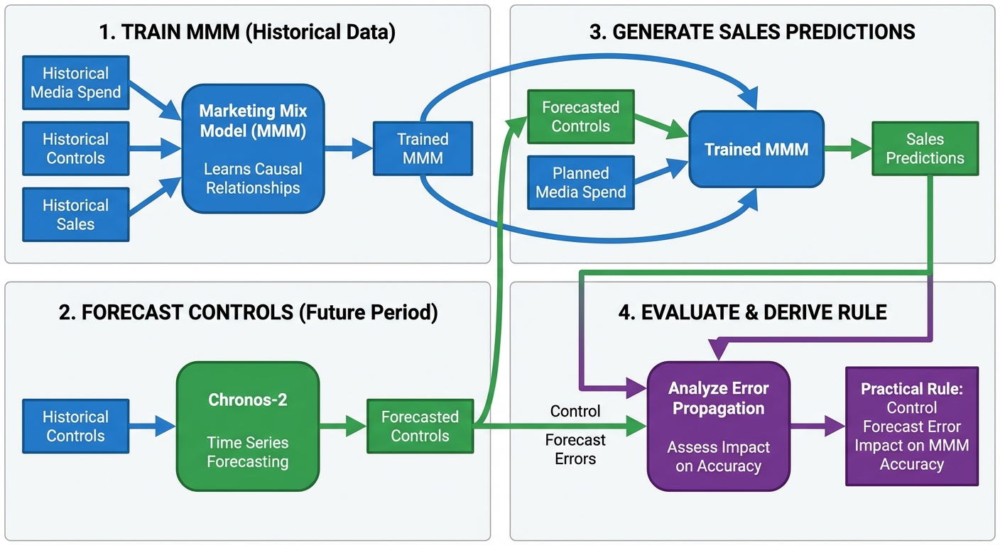
This tutorial presents a two-model technique:

1. Train an MMM on historical data to learn the causal relationships between media spend, controls, and sales

2. Use Chronos-2 to forecast the control variables into the future period

3. Combine the forecasted controls with planned media spend to generate sales predictions

4. Evaluate how forecast errors in controls propagate to sales predictions

This approach combines the best of two worlds: a general-purpose foundation model that accurately predict the future state of covariates, and a specialized Bayesian MMMs that explicitly model marketing effects and allow for causal interpretation.

We also derive a practical rule for estimating how much control forecast error affects MMM accuracy, helping practitioners set appropriate forecasting targets.

Background and Prerequisites

Before diving into the implementation, let’s briefly review the key concepts.

Media Mix Modeling (MMM)

MMM is a statistical technique used to measure the effectiveness of marketing channels. A typical MMM decomposes sales into:

\[ y_t = \text{baseline}_t + \sum_{c} f_c(\text{media}_{c,t}) + \sum_{j} \gamma_j z_{j,t} + \varepsilon_t \]

where:

• \(y_t\) is the target variable (e.g., sales) at time \(t\)

• \(f_c(\cdot)\) captures the nonlinear effect of media channel \(c\), typically including adstock (carryover effects) and saturation (diminishing returns)

• \(z_{j,t}\) are control variables (e.g., economic indicators, weather, holidays)

• \(\gamma_j\) are the coefficients for control variables

• \(\varepsilon_t\) is the error term

Control variables are external factors that influence sales but are not marketing activities. Including them helps isolate the true media effects from confounding factors.

For more information on MMM, see the example notebooks MMM Example Notebook and MMM End-to-End Case Study.

Foundational Time Series Models

Chronos-2 is a pretrained time series model developed by Amazon that can generate forecasts without task-specific training (zero-shot forecasting). Key characteristics:

• Handles univariate, multivariate, and covariate-informed forecasting

• Uses a group attention mechanism for in-context learning across related series

• Trained on diverse synthetic datasets to generalize across domains

In this tutorial, we use Chronos-2 to forecast control variables (employment, temperature) that exhibit predictable temporal patterns.

What This Tutorial Covers

• Setting up a multi-dimensional MMM with PyMC-Marketing

• Using Chronos-2 for zero-shot forecasting of control variables

• Evaluating how forecast errors propagate through the MMM

• Practical guidelines for setting forecast accuracy targets

What This Tutorial Does Not Cover

• MMM model selection and validation (see PyMC-Marketing documentation)

• Hyperparameter tuning for Chronos-2

• Budget optimization using MMM results

Setup

Warning

To run this notebook you can go to the original notebook https://github.com/lfiaschi/advanced-pymc-marketing-examples/blob/main/notebooks/07_chronos_pymc_marketing.ipynb and install the dependencies.

Import the required libraries. Key dependencies:

• pymc_marketing: Bayesian MMM implementation

• chronos: Amazon’s pretrained time series models

• polars: Fast DataFrame operations

• rich: Enhanced console output for tables and progress

import warnings
from pathlib import Path

import matplotlib.pyplot as plt
import numpy as np
import pandas as pd
import polars as pl
import torch
from chronos import Chronos2Pipeline
from rich import print as rprint
from rich.console import Console
from rich.table import Table

from pymc_marketing.mmm import GeometricAdstock, LogisticSaturation
from pymc_marketing.mmm.multidimensional import MMM

warnings.filterwarnings("ignore")

plt.rcParams["figure.figsize"] = [12, 7]
plt.rcParams["figure.dpi"] = 100

console = Console()

%load_ext autoreload
%autoreload 2
%config InlineBackend.figure_format = "retina"

/Users/juanitorduz/Documents/advanced-pymc-marketing-examples/.venv/lib/python3.12/site-packages/pymc_marketing/mmm/multidimensional.py:215: FutureWarning: This functionality is experimental and subject to change. If you encounter any issues or have suggestions, please raise them at: https://github.com/pymc-labs/pymc-marketing/issues/new
  warnings.warn(warning_msg, FutureWarning, stacklevel=1)

Load and Explore Data

We use a synthetic dataset designed to illustrate the key concepts. The data simulates a realistic MMM scenario with:

Variable	Description
week	Weekly timestamp (208 weeks, ~4 years)
state	US state identifier (50 states)
tv_spend	TV advertising spend
search_spend	Search advertising spend
avg_temp	Average temperature (control variable with seasonal pattern)
avg_employment	Employment rate (control variable with trend + noise)
y	Sales (target variable)

The sales variable was generated using a known MMM formula, which allows us to evaluate how well the approach recovers the true relationships. In practice, you would use real data where the ground truth is unknown.

# Load data
data_path = Path(
    "https://raw.githubusercontent.com/lfiaschi/advanced-pymc-marketing-examples/main/data/mmm-chronos/mmm_chronos_data.csv"
)
df = pl.read_csv(data_path).with_columns(pl.col("week").str.to_date())

rprint("[bold green]Data loaded successfully[/bold green]")
rprint(f"Shape: {df.shape[0]} rows × {df.shape[1]} columns")
rprint(f"Date range: {df['week'].min()} to {df['week'].max()}")
rprint(f"Number of states: {df['state'].n_unique()}")
rprint(f"\nColumns: {df.columns}")


# Preview first few rows
def display_data_preview(df: pl.DataFrame, n: int = 5) -> None:
    """Display a preview of the dataframe using Rich Table."""
    table = Table(title="Data Preview", show_header=True, header_style="bold magenta")

    # Add columns
    for col in df.columns:
        table.add_column(str(col))

    # Add rows
    for row in df.head(n).iter_rows():
        table.add_row(*[str(v) for v in row])

    console.print(table)


display_data_preview(df)

Data loaded successfully

Shape: 10400 rows × 7 columns

Date range: 2020-01-12 to 2023-12-31

Number of states: 50

Columns: ['week', 'state', 'avg_temp', 'avg_employment', 'tv_spend', 'search_spend', 'y']

                                        Data Preview                                        
┏━━━━━━━━━━━━┳━━━━━━━━━━━━┳━━━━━━━━━━┳━━━━━━━━━━━━━━━━┳━━━━━━━━━━┳━━━━━━━━━━━━━━┳━━━━━━━━━━┓
┃ week       ┃ state      ┃ avg_temp ┃ avg_employment ┃ tv_spend ┃ search_spend ┃ y        ┃
┡━━━━━━━━━━━━╇━━━━━━━━━━━━╇━━━━━━━━━━╇━━━━━━━━━━━━━━━━╇━━━━━━━━━━╇━━━━━━━━━━━━━━╇━━━━━━━━━━┩
│ 2020-01-12 │ New Jersey │ 40.2     │ 0.9531         │ 15201.77 │ 6518.94      │ 47344.14 │
│ 2020-01-19 │ New Jersey │ 32.6     │ 0.9528         │ 14082.6  │ 5496.16      │ 47458.42 │
│ 2020-01-26 │ New Jersey │ 35.8     │ 0.9533         │ 13779.59 │ 3919.59      │ 47367.3  │
│ 2020-02-02 │ New Jersey │ 41.4     │ 0.9552         │ 14238.66 │ 3133.07      │ 47360.27 │
│ 2020-02-09 │ New Jersey │ 37.1     │ 0.9611         │ 15145.33 │ 2515.58      │ 47372.65 │
└────────────┴────────────┴──────────┴────────────────┴──────────┴──────────────┴──────────┘

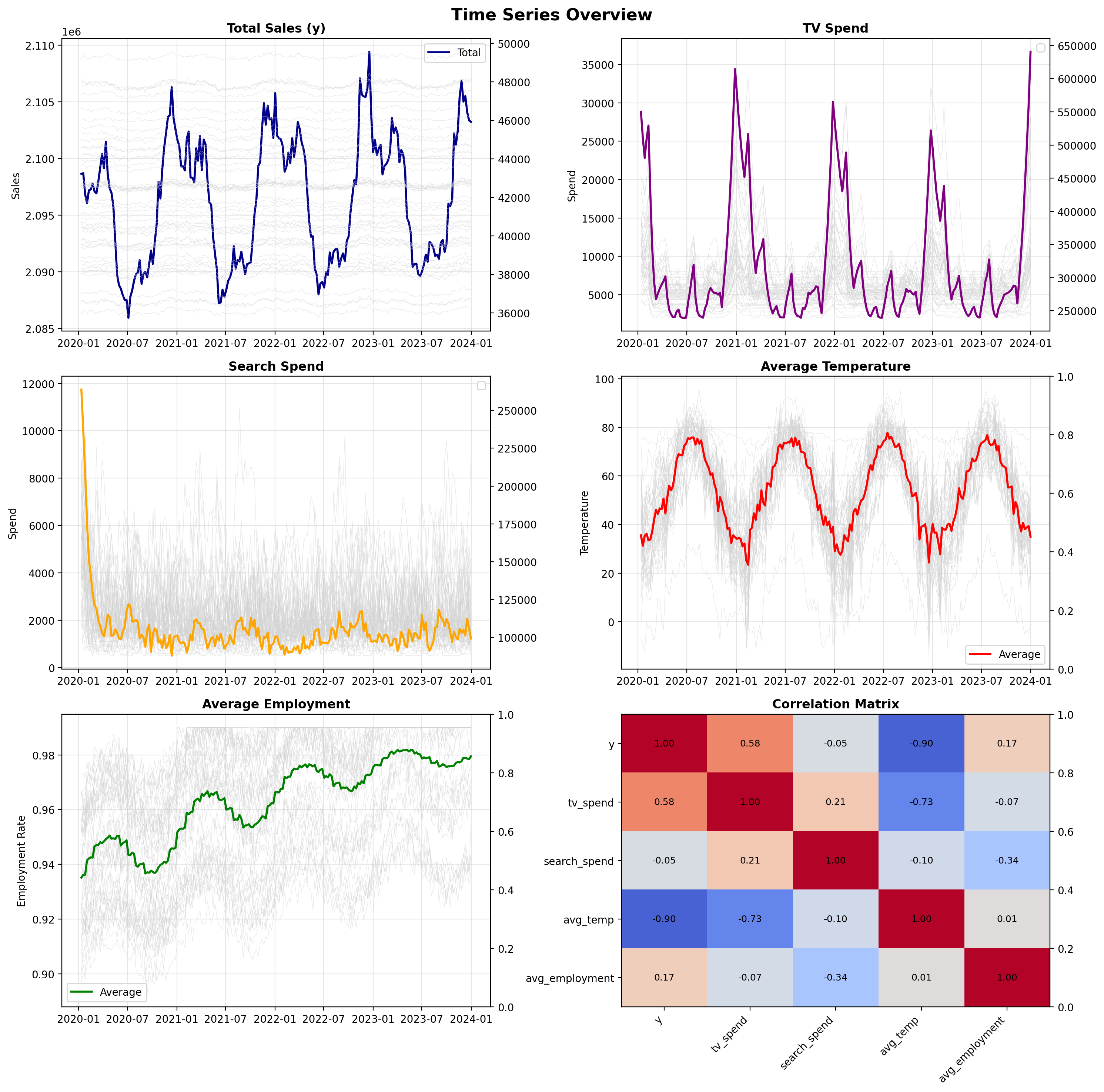
Visualize Time Series Patterns

Before modeling, we examine the temporal patterns in our data. Key observations to look for:

• Seasonality: Temperature shows clear annual cycles; employment may have subtler patterns

• Trends: Employment rates may drift over time

• Correlation structure: Understanding how variables relate helps interpret model results

The visualization below shows aggregated time series (bold lines) with individual state series in the background (gray lines). This reveals both the overall patterns and the cross-sectional variation.

Show code cell source

Hide code cell source

def plot_time_series(df: pl.DataFrame) -> None:
    """Plot time series for key variables with all states in background."""
    # Aggregate by week (sum across states for spend/sales, mean for controls)
    df_agg = (
        df.group_by("week")
        .agg(
            [
                pl.col("y").sum().alias("y"),
                pl.col("tv_spend").sum().alias("tv_spend"),
                pl.col("search_spend").sum().alias("search_spend"),
                pl.col("avg_temp").mean().alias("avg_temp"),
                pl.col("avg_employment").mean().alias("avg_employment"),
            ]
        )
        .sort("week")
    )

    fig, axes = plt.subplots(3, 2, figsize=(15, 15))
    axes_twin = np.array([ax.twinx() for ax in axes.flatten()]).reshape(axes.shape)
    fig.suptitle("Time Series Overview", fontsize=16, fontweight="bold")

    # Get all unique states
    states = df["state"].unique().to_list()

    # Sales - All states + Total
    for state in states:
        df_state = df.filter(pl.col("state") == state).sort("week")
        axes_twin[0, 0].plot(
            df_state["week"], df_state["y"], color="lightgray", linewidth=0.5, alpha=0.5
        )
    axes[0, 0].plot(
        df_agg["week"], df_agg["y"], color="darkblue", linewidth=2, label="Total"
    )
    axes[0, 0].set_title("Total Sales (y)", fontweight="bold")
    axes[0, 0].set_ylabel("Sales")
    axes[0, 0].legend()
    axes[0, 0].grid(alpha=0.3)

    # TV Spend - All states + Total
    for state in states:
        df_state = df.filter(pl.col("state") == state).sort("week")
        axes[0, 1].plot(
            df_state["week"],
            df_state["tv_spend"],
            color="lightgray",
            linewidth=0.5,
            alpha=0.5,
        )
    axes_twin[0, 1].plot(
        df_agg["week"], df_agg["tv_spend"], color="purple", linewidth=2, label="Total"
    )
    axes[0, 1].set_title("TV Spend", fontweight="bold")
    axes[0, 1].set_ylabel("Spend")
    axes[0, 1].legend()
    axes[0, 1].grid(alpha=0.3)

    # Search Spend - All states + Total
    for state in states:
        df_state = df.filter(pl.col("state") == state).sort("week")
        axes[1, 0].plot(
            df_state["week"],
            df_state["search_spend"],
            color="lightgray",
            linewidth=0.5,
            alpha=0.5,
        )
    axes_twin[1, 0].plot(
        df_agg["week"],
        df_agg["search_spend"],
        color="orange",
        linewidth=2,
        label="Total",
    )
    axes[1, 0].set_title("Search Spend", fontweight="bold")
    axes[1, 0].set_ylabel("Spend")
    axes[1, 0].legend()
    axes[1, 0].grid(alpha=0.3)

    # Temperature - All states + Average
    for state in states:
        df_state = df.filter(pl.col("state") == state).sort("week")
        axes[1, 1].plot(
            df_state["week"],
            df_state["avg_temp"],
            color="lightgray",
            linewidth=0.5,
            alpha=0.5,
        )
    axes[1, 1].plot(
        df_agg["week"], df_agg["avg_temp"], color="red", linewidth=2, label="Average"
    )
    axes[1, 1].set_title("Average Temperature", fontweight="bold")
    axes[1, 1].set_ylabel("Temperature")
    axes[1, 1].legend()
    axes[1, 1].grid(alpha=0.3)

    # Employment - All states + Average
    for state in states:
        df_state = df.filter(pl.col("state") == state).sort("week")
        axes[2, 0].plot(
            df_state["week"],
            df_state["avg_employment"],
            color="lightgray",
            linewidth=0.5,
            alpha=0.5,
        )
    axes[2, 0].plot(
        df_agg["week"],
        df_agg["avg_employment"],
        color="green",
        linewidth=2,
        label="Average",
    )
    axes[2, 0].set_title("Average Employment", fontweight="bold")
    axes[2, 0].set_ylabel("Employment Rate")
    axes[2, 0].legend()
    axes[2, 0].grid(alpha=0.3)

    # Correlation heatmap
    corr_data = (
        df_agg.select(["y", "tv_spend", "search_spend", "avg_temp", "avg_employment"])
        .to_pandas()
        .corr()
    )

    axes[2, 1].imshow(corr_data, cmap="coolwarm", vmin=-1, vmax=1, aspect="auto")
    axes[2, 1].set_xticks(range(len(corr_data.columns)))
    axes[2, 1].set_yticks(range(len(corr_data.columns)))
    axes[2, 1].set_xticklabels(corr_data.columns, rotation=45, ha="right")
    axes[2, 1].set_yticklabels(corr_data.columns)
    axes[2, 1].set_title("Correlation Matrix", fontweight="bold")

    # Add correlation values
    for i in range(len(corr_data.columns)):
        for j in range(len(corr_data.columns)):
            axes[2, 1].text(
                j,
                i,
                f"{corr_data.iloc[i, j]:.2f}",
                ha="center",
                va="center",
                color="black",
                fontsize=9,
            )

    plt.tight_layout()
    plt.show()


plot_time_series(df)

rprint("[bold green]✓[/bold green] Time series visualization complete")

✓ Time series visualization complete

# Create summary table of average spend by state
non_null_y_count = df.filter(pl.col("y").is_not_null()).shape[0]
total_count = df.shape[0]
rprint(
    f"[yellow]Data check:[/yellow] {non_null_y_count} non-null sales values out of {total_count} total rows"
)

# Aggregate spend and sales data
spend_summary = (
    df.group_by("state")
    .agg(
        [
            pl.col("tv_spend").mean().alias("Avg TV Spend"),
            pl.col("search_spend").mean().alias("Avg Search Spend"),
            (pl.col("tv_spend") + pl.col("search_spend"))
            .mean()
            .alias("Avg Total Spend"),
            pl.col("y").mean().alias("Avg Sales"),
        ]
    )
    .sort("Avg Total Spend", descending=True)
)

# Display using Rich table
table = Table(
    title="Average Media Spend by State", show_header=True, header_style="bold magenta"
)
table.add_column("State", style="cyan", no_wrap=True)
table.add_column("Avg TV Spend", justify="right", style="green")
table.add_column("Avg Search Spend", justify="right", style="blue")
table.add_column("Avg Total Spend", justify="right", style="yellow")
table.add_column("Avg Sales", justify="right", style="magenta")

for row in spend_summary.iter_rows(named=True):
    avg_sales = row.get("Avg Sales")
    sales_str = (
        f"${avg_sales:,.2f}"
        if avg_sales is not None and not np.isnan(avg_sales)
        else "$nan"
    )

    table.add_row(
        row["state"],
        f"${row['Avg TV Spend']:,.2f}",
        f"${row['Avg Search Spend']:,.2f}",
        f"${row['Avg Total Spend']:,.2f}",
        sales_str,
    )

console.print(table)
rprint(
    f"\n[bold green]✓[/bold green] Average spend summary for {len(spend_summary)} states"
)

Data check: 10400 non-null sales values out of 10400 total rows

                           Average Media Spend by State                            
┏━━━━━━━━━━━━━━━━┳━━━━━━━━━━━━━━┳━━━━━━━━━━━━━━━━━━┳━━━━━━━━━━━━━━━━━┳━━━━━━━━━━━━┓
┃ State          ┃ Avg TV Spend ┃ Avg Search Spend ┃ Avg Total Spend ┃  Avg Sales ┃
┡━━━━━━━━━━━━━━━━╇━━━━━━━━━━━━━━╇━━━━━━━━━━━━━━━━━━╇━━━━━━━━━━━━━━━━━╇━━━━━━━━━━━━┩
│ Texas          │   $13,119.02 │        $3,488.64 │      $16,607.65 │ $44,563.98 │
│ New York       │   $11,110.87 │        $3,232.43 │      $14,343.30 │ $40,571.07 │
│ North Carolina │   $10,442.48 │        $2,585.67 │      $13,028.15 │ $36,077.00 │
│ California     │   $10,168.02 │        $2,853.00 │      $13,021.02 │ $46,568.23 │
│ Virginia       │   $10,028.41 │        $2,776.01 │      $12,804.43 │ $41,167.96 │
│ Florida        │    $8,662.81 │        $3,671.72 │      $12,334.53 │ $46,058.95 │
│ Michigan       │    $9,526.88 │        $2,208.14 │      $11,735.02 │ $43,541.15 │
│ Washington     │    $9,266.80 │        $2,318.26 │      $11,585.06 │ $45,027.23 │
│ Ohio           │    $8,592.62 │        $2,652.97 │      $11,245.59 │ $47,810.30 │
│ Arizona        │    $8,540.73 │        $2,396.62 │      $10,937.35 │ $37,023.59 │
│ Massachusetts  │    $8,453.45 │        $2,237.68 │      $10,691.13 │ $38,583.65 │
│ Maryland       │    $7,818.03 │        $2,811.47 │      $10,629.50 │ $38,382.23 │
│ Georgia        │    $8,134.42 │        $2,452.15 │      $10,586.57 │ $49,311.96 │
│ New Jersey     │    $7,815.47 │        $2,533.53 │      $10,349.00 │ $47,395.09 │
│ Tennessee      │    $7,057.37 │        $2,991.86 │      $10,049.22 │ $36,561.22 │
│ Pennsylvania   │    $7,011.23 │        $2,591.39 │       $9,602.62 │ $36,522.99 │
│ Illinois       │    $6,918.14 │        $2,527.18 │       $9,445.32 │ $41,458.58 │
│ Indiana        │    $6,783.76 │        $2,466.04 │       $9,249.80 │ $42,577.13 │
│ Colorado       │    $7,241.18 │        $1,940.75 │       $9,181.93 │ $42,659.58 │
│ Alabama        │    $6,741.88 │        $2,079.21 │       $8,821.09 │ $42,608.70 │
│ Utah           │    $6,296.27 │        $2,010.29 │       $8,306.56 │ $42,697.24 │
│ Minnesota      │    $5,863.78 │        $2,423.63 │       $8,287.42 │ $43,886.93 │
│ Wisconsin      │    $6,133.24 │        $2,137.53 │       $8,270.77 │ $38,823.46 │
│ Missouri       │    $6,118.05 │        $2,140.19 │       $8,258.24 │ $41,646.40 │
│ South Carolina │    $5,852.71 │        $2,351.09 │       $8,203.80 │ $41,826.13 │
│ Louisiana      │    $5,740.20 │        $2,419.14 │       $8,159.34 │ $40,197.79 │
│ Kentucky       │    $6,206.40 │        $1,788.57 │       $7,994.97 │ $40,409.35 │
│ Oklahoma       │    $5,672.99 │        $2,252.08 │       $7,925.07 │ $44,168.58 │
│ Nevada         │    $5,819.73 │        $1,861.21 │       $7,680.94 │ $39,540.26 │
│ Oregon         │    $5,478.41 │        $2,163.56 │       $7,641.97 │ $45,645.29 │
│ Arkansas       │    $5,386.22 │        $2,204.78 │       $7,590.99 │ $37,938.06 │
│ Connecticut    │    $5,363.95 │        $2,102.55 │       $7,466.50 │ $38,423.62 │
│ Rhode Island   │    $5,907.17 │        $1,538.08 │       $7,445.26 │ $40,347.66 │
│ Iowa           │    $5,342.37 │        $2,025.32 │       $7,367.69 │ $42,526.36 │
│ Mississippi    │    $5,230.54 │        $2,019.36 │       $7,249.91 │ $40,926.04 │
│ Kansas         │    $4,852.29 │        $1,849.73 │       $6,702.03 │ $39,698.36 │
│ South Dakota   │    $4,745.62 │        $1,605.33 │       $6,350.95 │ $47,893.26 │
│ New Mexico     │    $4,455.08 │        $1,806.37 │       $6,261.46 │ $38,157.56 │
│ Nebraska       │    $4,830.44 │        $1,383.80 │       $6,214.24 │ $39,691.08 │
│ Montana        │    $4,816.72 │        $1,270.47 │       $6,087.19 │ $40,588.26 │
│ Idaho          │    $4,088.37 │        $1,679.87 │       $5,768.25 │ $47,878.32 │
│ West Virginia  │    $4,149.01 │        $1,392.10 │       $5,541.11 │ $42,520.13 │
│ North Dakota   │    $4,425.96 │        $1,111.71 │       $5,537.67 │ $38,079.59 │
│ Hawaii         │    $4,070.03 │        $1,300.52 │       $5,370.54 │ $39,482.65 │
│ Maine          │    $3,686.36 │        $1,569.44 │       $5,255.80 │ $42,625.58 │
│ Vermont        │    $4,104.00 │        $1,000.38 │       $5,104.38 │ $42,779.92 │
│ New Hampshire  │    $3,593.72 │        $1,342.33 │       $4,936.04 │ $39,465.69 │
│ Delaware       │    $3,057.86 │        $1,076.01 │       $4,133.87 │ $44,586.82 │
│ Alaska         │    $2,533.31 │        $1,014.69 │       $3,548.00 │ $44,210.96 │
│ Wyoming        │    $2,276.67 │          $898.41 │       $3,175.08 │ $45,259.07 │
└────────────────┴──────────────┴──────────────────┴─────────────────┴────────────┘

✓ Average spend summary for 50 states

Understanding Error Propagation: Theory

Before implementing the approach, it’s useful to understand how forecast errors in control variables affect MMM predictions. This section derives a practical rule for estimating the impact.

The Core Question

When we replace true control values \(z\) with forecasts \(\tilde{z}\), how much does the MMM prediction error increase?

Key Insight

The answer depends on two factors:

1. Control share: How much do controls contribute to the predicted sales?

2. Forecast accuracy: How accurate are the control forecasts (measured by MAPE)?

The Rule of Thumb

Incremental MMM MAPE ≈ Control Share × Control MAPE

For example:

• If controls explain 30% of sales variation

• And control forecast MAPE is 10%

• Then expect roughly 3% additional MAPE in sales predictions

Practical Guidelines

Control Share	Recommended Control MAPE	Expected Impact
≤ 20%	Any reasonable	Negligible (≤ 2% MAPE)
30-50%	≤ 10%	Moderate (3-5% MAPE)
> 50%	≤ 5%	Each 1% adds ~0.5-1% MAPE

Mathematical Derivation (Optional)

For readers interested in the derivation, the MMM prediction with controls is:

\[ \hat{y}_i = f(x_i) + \sum_{j=1}^p \gamma_j z_{ij} \]

where \(f(x_i)\) is the media contribution and \(\gamma_j z_{ij}\) is the control contribution. When we substitute forecasted controls \(\tilde{z}_{ij}\), the prediction changes by:

\[ \Delta \hat{y}_i = \sum_j \gamma_j (\tilde{z}_{ij} - z_{ij}) = \sum_j \gamma_j z_{ij} \varepsilon_{ij} \]

where \(\varepsilon_{ij} = (\tilde{z}_{ij} - z_{ij})/z_{ij}\) is the relative forecast error.

The resulting MAPE increase is bounded by:

\[ \text{MAPE}_y^{(\text{from controls})} \leq \frac{1}{n} \sum_i \left[ \sum_j \frac{|\gamma_j| |z_{ij}|}{|y_i|} m_j \right] \]

where \(m_j\) is the MAPE of control \(j\). The term \(|\gamma_j| |z_{ij}| / |y_i|\) represents the control share—the fraction of sales explained by control \(j\).

When all controls have similar forecast accuracy \(M_z\), this simplifies to:

\[ \text{MAPE}_y^{(\text{from controls})} \approx M_z \times \text{(Average Control Share)} \]

This derivation justifies the rule of thumb and helps practitioners set appropriate forecasting targets.

Step 1: Split Data into Training and Test Sets

We use a temporal split to simulate a realistic forecasting scenario:

• Training period (Years 1-3): Used to fit the MMM and learn the relationships between media, controls, and sales

• Test period (Year 4): Held out to evaluate predictions—we pretend we don’t know the control values for this period

This split allows us to measure how well the approach works when control variables must be forecasted rather than observed.

Practical Tip: When choosing your split point, ensure the training period captures at least one full cycle of any seasonal patterns in your control variables. For annual seasonality (like temperature), this means at least 1-2 years of training data.

# Split data
split_date = pl.date(2023, 1, 1)
train_data = df.filter(pl.col("week") < split_date)
test_data = df.filter(pl.col("week") >= split_date)

rprint(
    f"[bold cyan]Training data:[/bold cyan] {train_data.shape[0]} rows ({train_data['week'].min()} to {train_data['week'].max()})"  # noqa: E501
)
rprint(
    f"[bold cyan]Test data:[/bold cyan] {test_data.shape[0]} rows ({test_data['week'].min()} to {test_data['week'].max()})"  # noqa: E501
)

# Define column names
channel_columns = ["tv_spend", "search_spend"]
control_columns = ["avg_employment", "avg_temp"]
date_column = "week"

Training data: 7750 rows (2020-01-12 to 2022-12-25)

Test data: 2650 rows (2023-01-01 to 2023-12-31)

Step 2: Fit the MMM on Training Data

We fit a PyMC-Marketing MMM to the training data. The model learns:

• Media effects: How TV and search spend influence sales, including adstock (carryover) and saturation (diminishing returns)

• Control effects: The coefficients \(\gamma_j\) for employment and temperature

• Seasonality: Yearly patterns captured via Fourier terms

The model uses a multi-dimensional structure with dims=("state",) to share information across states while allowing state-specific scaling. This is particularly useful when you have panel data with multiple geographic units.

Practical Tip: The sampler configuration below uses reduced settings for faster execution in this tutorial. For production use, increase draws to 1000+ and use 4 chains to ensure proper convergence. Always check rhat values and effective sample sizes in your diagnostics.

%%time

# 1) To pandas and basic hygiene
train_df = train_data.to_pandas()
train_df[date_column] = pd.to_datetime(train_df[date_column])
train_df = train_df.sort_values(["state", date_column]).reset_index(drop=True)

# 2) Build X (features) and y (target)
feature_cols = [date_column, "state", *channel_columns, *control_columns]
X = train_df[feature_cols].copy()
y = train_df["y"]

assert "state" in X.columns, "state must be present in X"  # noqa: S101

# 3) Configure sampling for faster execution in this tutorial
# For production, increase draws to 1000+ and verify convergence diagnostics
sampler_config = {
    "draws": 200,
    "tune": 1_500,
    "chains": 8,
    "cores": 8,
    "target_accept": 0.95,
    "random_seed": 42,
}

rprint("[yellow]Training MMM with reduced sampling for faster execution...[/yellow]")
rprint(
    "[dim]For production use, increase draws to 1000+ and use 4 chains for better convergence[/dim]"
)

# 4) Define and fit the multidimensional MMM
mmm = MMM(
    date_column=date_column,
    channel_columns=channel_columns,
    adstock=GeometricAdstock(l_max=13),
    saturation=LogisticSaturation(),
    yearly_seasonality=3,
    control_columns=control_columns,
    target_column="y",
    dims=("state",),
    sampler_config=sampler_config,  # Pass sampler_config to constructor
)

mmm.fit(X, y)

rprint("[bold green]✓ MMM training complete[/bold green]")

Training MMM with reduced sampling for faster execution...

For production use, increase draws to 1000+ and use 4 chains for better convergence

Initializing NUTS using jitter+adapt_diag...
Multiprocess sampling (8 chains in 8 jobs)
NUTS: [intercept_contribution, adstock_alpha, saturation_lam, saturation_beta, gamma_control, gamma_fourier, y_sigma]

Sampling 8 chains for 1_500 tune and 200 draw iterations (12_000 + 1_600 draws total) took 1206 seconds.
Chain 0 reached the maximum tree depth. Increase `max_treedepth`, increase `target_accept` or reparameterize.
Chain 2 reached the maximum tree depth. Increase `max_treedepth`, increase `target_accept` or reparameterize.
The rhat statistic is larger than 1.01 for some parameters. This indicates problems during sampling. See https://arxiv.org/abs/1903.08008 for details
The effective sample size per chain is smaller than 100 for some parameters.  A higher number is needed for reliable rhat and ess computation. See https://arxiv.org/abs/1903.08008 for details

✓ MMM training complete

CPU times: user 3.86 s, sys: 620 ms, total: 4.48 s
Wall time: 20min 9s

Step 3: Forecast Control Variables with Chronos-2

With the MMM trained, we now need forecasts of the control variables for the test period. This is where Chronos-2 comes in.

Chronos-2 is a pretrained time series model that can generate forecasts without any task-specific training. We provide it with the historical control variable data, and it produces forecasts for the next 52 weeks.

Key aspects of our approach:

• Multi-target forecasting: We forecast both employment and temperature simultaneously

• Per-state forecasts: Each state gets its own forecast based on its historical pattern

• Uncertainty quantification: Chronos-2 provides prediction intervals (10th, 50th, 90th percentiles)

The function below handles the data preparation, model loading, and forecast generation.

Practical Tip: If you have access to a GPU, set device="cuda" for faster inference. For large-scale applications with many series, consider batching the forecasts to manage memory usage.

Show code cell source

Hide code cell source

def forecast_controls_with_chronos2(
    train_data: pl.DataFrame,
    control_cols: list[str],
    prediction_length: int = 52,
    device: str = "cpu",
) -> pl.DataFrame:
    quantile_levels = (0.1, 0.5, 0.9)

    # Force single-threaded execution for PyTorch DataLoader to avoid multiprocessing issues in notebooks
    torch.set_num_threads(1)

    # 1) Load Chronos-2
    pipeline = Chronos2Pipeline.from_pretrained(
        "s3://autogluon/chronos-2",
        device_map=("cuda" if device == "cuda" else "cpu"),
        dtype=torch.bfloat16,
    )

    # 2) Prepare global context DataFrame for Chronos-2 (pandas I/O)
    needed = ["state", "week", *control_cols]
    df = (
        train_data.select(needed)
        .sort(["state", "week"])
        .to_pandas()
        .rename(columns={"state": "id", "week": "timestamp"})
    )

    # Basic cleaning for targets
    for c in control_cols:
        s = df[c].astype("float32")
        if s.isna().any():
            mean_val = float(s.mean()) if pd.notna(s.mean()) else 0.0
            s = s.fillna(mean_val)
        df[c] = s

    # 3) One global call with multiple IDs and multiple targets
    # Force num_workers=0 to avoid multiprocessing issues
    q_levels = list(quantile_levels) if quantile_levels else None
    pred_df = pipeline.predict_df(
        df,
        prediction_length=prediction_length,
        quantile_levels=q_levels,
        id_column="id",
        timestamp_column="timestamp",
        target=control_cols,  # multi-output
    )
    print(pred_df.columns.tolist())
    # pred_df columns include: ['id','timestamp','target','predictions', *quantiles...]

    # 4) Pivot to wide per state-week for mean prediction
    mean_wide = (
        pred_df.pivot(
            index=["timestamp", "id"], columns="target_name", values="predictions"
        )
        .reset_index()
        .rename(columns={c: f"{c}_forecast" for c in control_cols})
    )

    # 5) Pivot quantiles to wide and merge
    merged = mean_wide
    if q_levels:
        for q in q_levels:
            qcol = f"{q:.1f}" if isinstance(q, float) else str(q)
            if qcol in pred_df.columns:
                qw = (
                    pred_df.pivot(
                        index=["timestamp", "id"], columns="target_name", values=qcol
                    )
                    .reset_index()
                    .rename(
                        columns={
                            c: f"{c}_q{round(float(q) * 100):02d}" for c in control_cols
                        }
                    )
                )
                merged = merged.merge(qw, on=["timestamp", "id"], how="left")

    # 6) Back to Polars, rename to original keys, tidy ordering
    result = (
        pl.from_pandas(merged)
        .rename({"timestamp": "week", "id": "state"})
        .sort(["state", "week"])
    )

    return result


rprint(
    "[yellow]Generating Chronos2 forecasts (this may take a few minutes)...[/yellow]"
)
control_forecasts = forecast_controls_with_chronos2(
    train_data,
    control_columns,
    prediction_length=52,
    device="cpu",  # Change to "cuda" if GPU available
)
rprint("[bold green]✓ Chronos2 forecasts complete[/bold green]")

Generating Chronos2 forecasts (this may take a few minutes)...

['id', 'timestamp', 'target_name', 'predictions', '0.1', '0.5', '0.9']

✓ Chronos2 forecasts complete

control_forecasts

shape: (2_600, 10)

week	state	avg_employment_forecast	avg_temp_forecast	avg_employment_q10	avg_temp_q10	avg_employment_q50	avg_temp_q50	avg_employment_q90	avg_temp_q90
datetime[ns]	str	f32	f32	f32	f32	f32	f32	f32	f32
2023-01-01 00:00:00	"Alabama"	0.984375	46.75	0.980469	39.5	0.984375	46.75	0.988281	54.0
2023-01-08 00:00:00	"Alabama"	0.984375	46.5	0.984375	39.0	0.984375	46.5	0.988281	53.75
2023-01-15 00:00:00	"Alabama"	0.988281	46.5	0.984375	38.5	0.988281	46.5	0.9921875	54.0
2023-01-22 00:00:00	"Alabama"	0.988281	47.25	0.988281	39.5	0.988281	47.25	0.9921875	54.5
2023-01-29 00:00:00	"Alabama"	0.9921875	47.75	0.988281	41.0	0.9921875	47.75	0.996094	55.25
…	…	…	…	…	…	…	…	…	…
2023-11-26 00:00:00	"Wyoming"	0.988281	19.125	0.984375	6.03125	0.988281	19.125	0.988281	29.125
2023-12-03 00:00:00	"Wyoming"	0.988281	17.25	0.980469	5.71875	0.988281	17.25	0.988281	26.125
2023-12-10 00:00:00	"Wyoming"	0.988281	15.5625	0.980469	3.875	0.988281	15.5625	0.988281	23.875
2023-12-17 00:00:00	"Wyoming"	0.988281	14.625	0.980469	2.921875	0.988281	14.625	0.988281	22.875
2023-12-24 00:00:00	"Wyoming"	0.988281	13.5	0.980469	1.6171875	0.988281	13.5	0.988281	22.0

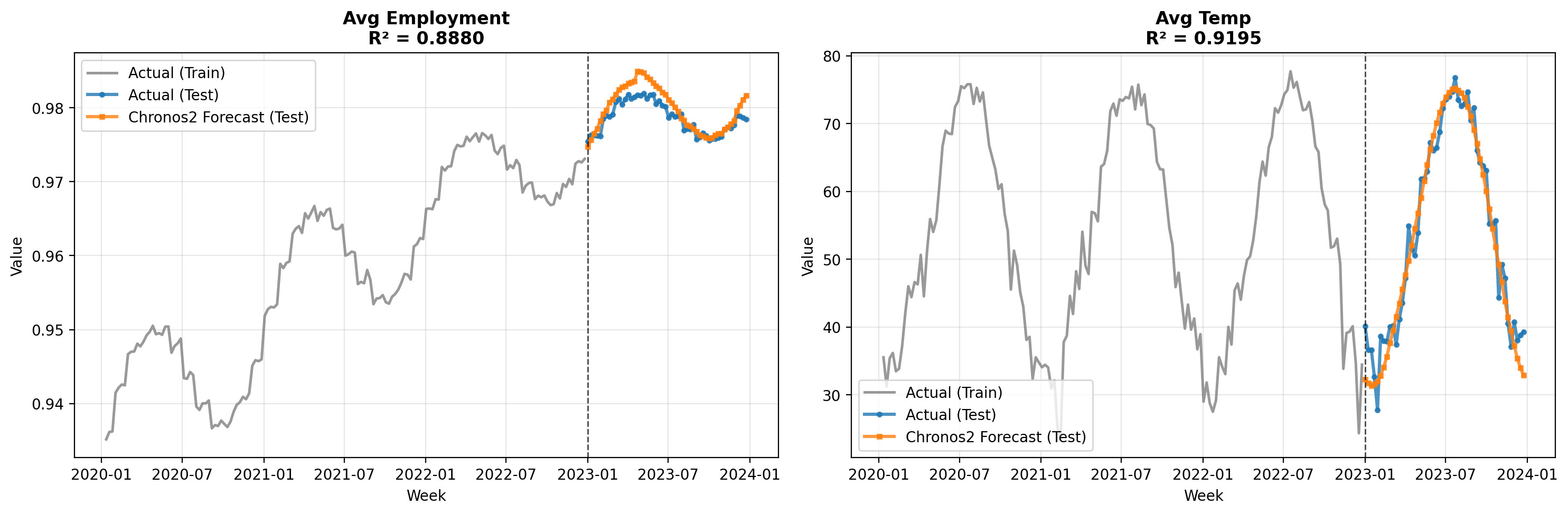
Evaluate Forecast Accuracy

Before using the forecasted controls in the MMM, we evaluate how well Chronos-2 predicted the actual values. This is important because, as we derived earlier, the control forecast MAPE directly affects the MMM prediction accuracy.

The metrics below show the forecast accuracy for each control variable. Pay attention to the MAPE values—these will help us estimate the expected degradation in MMM predictions.

Practical Tip: If the control forecast MAPE is unacceptably high, consider: (1) using a different forecasting model, (2) incorporating external information (e.g., economic forecasts), or (3) reducing the forecast horizon.

Show code cell source

Hide code cell source

# Merge forecasts with actual test data
test_data_pd = test_data.to_pandas()
test_controls_actual = test_data_pd[["week", "state", *control_columns]].copy()

# Also prepare TRAINING actuals for plotting
# Use existing train_df prepared earlier
train_controls_actual = train_df[["week", "state", *control_columns]].copy()

# Convert forecasts to pandas
control_forecasts_pd = control_forecasts.to_pandas()

# Merge actual and forecasted (TEST period)
comparison_data = test_controls_actual.merge(
    control_forecasts_pd, on=["week", "state"], how="inner"
)


# Calculate metrics for each control variable
def calculate_metrics(actual: np.ndarray, predicted: np.ndarray) -> dict:
    """Calculate accuracy metrics."""
    mae = np.mean(np.abs(actual - predicted))
    rmse = np.sqrt(np.mean((actual - predicted) ** 2))
    mape = np.mean(np.abs((actual - predicted) / (np.abs(actual) + 1e-8))) * 100
    r2 = 1 - (
        np.sum((actual - predicted) ** 2) / np.sum((actual - np.mean(actual)) ** 2)
    )
    return {"MAE": mae, "RMSE": rmse, "MAPE": mape, "R²": r2}


# Compute metrics per control variable (TEST period)
rprint("[bold cyan]Chronos2 Forecast Accuracy Metrics[/bold cyan]")
metrics_summary = {}

for control in control_columns:
    actual_col = control
    forecast_col = f"{control}_forecast"

    actual_values = comparison_data[actual_col].values
    forecast_values = comparison_data[forecast_col].values

    # Filter out NaN values
    valid_mask = ~(np.isnan(actual_values) | np.isnan(forecast_values))
    actual_values = actual_values[valid_mask]
    forecast_values = forecast_values[valid_mask]

    metrics = calculate_metrics(actual_values, forecast_values)
    metrics_summary[control] = metrics

# Display metrics table
metrics_table = Table(
    title="Control Variable Forecast Accuracy",
    show_header=True,
    header_style="bold magenta",
)
metrics_table.add_column("Control Variable", style="cyan")
metrics_table.add_column("MAE", justify="right", style="green")
metrics_table.add_column("RMSE", justify="right", style="yellow")
metrics_table.add_column("MAPE (%)", justify="right", style="blue")
metrics_table.add_column("R²", justify="right", style="magenta")

for control, metrics in metrics_summary.items():
    metrics_table.add_row(
        control,
        f"{metrics['MAE']:.4f}",
        f"{metrics['RMSE']:.4f}",
        f"{metrics['MAPE']:.2f}",
        f"{metrics['R²']:.4f}",
    )

console.print(metrics_table)

# Plot forecast vs actual (TEST) and actuals (TRAIN) for each control variable
fig, axes = plt.subplots(1, len(control_columns), figsize=(15, 5))
if len(control_columns) == 1:
    axes = [axes]

# Ensure datetime types and compute split timestamp from test_data
train_controls_actual["week"] = pd.to_datetime(train_controls_actual["week"])
comparison_data["week"] = pd.to_datetime(comparison_data["week"])
split_ts = pd.to_datetime(test_data_pd["week"].min())

for idx, control in enumerate(control_columns):
    actual_col = control
    forecast_col = f"{control}_forecast"

    # Aggregate by week (mean across states), sort by date
    train_weekly = train_controls_actual.groupby("week")[actual_col].mean().sort_index()
    test_actual_weekly = comparison_data.groupby("week")[actual_col].mean().sort_index()
    forecast_weekly = comparison_data.groupby("week")[forecast_col].mean().sort_index()

    # Plot with proper dates on x-axis
    axes[idx].plot(
        train_weekly.index,
        train_weekly.values,
        label="Actual (Train)",
        linewidth=1.8,
        color="gray",
        alpha=0.8,
    )
    axes[idx].plot(
        test_actual_weekly.index,
        test_actual_weekly.values,
        label="Actual (Test)",
        linewidth=2.2,
        marker="o",
        markersize=3,
        alpha=0.8,
    )
    axes[idx].plot(
        forecast_weekly.index,
        forecast_weekly.values,
        label="Chronos2 Forecast (Test)",
        linewidth=2.2,
        marker="s",
        markersize=3,
        alpha=0.8,
    )

    # Mark train/test split
    axes[idx].axvline(split_ts, color="black", linestyle="--", linewidth=1, alpha=0.7)

    axes[idx].set_title(
        f"{control.replace('_', ' ').title()}\nR² = {metrics_summary[control]['R²']:.4f}",
        fontweight="bold",
    )
    axes[idx].set_xlabel("Week")
    axes[idx].set_ylabel("Value")
    axes[idx].legend()
    axes[idx].grid(alpha=0.3)

plt.tight_layout()
plt.show()

rprint("[bold green]✓ Forecast evaluation complete[/bold green]")

Chronos2 Forecast Accuracy Metrics

            Control Variable Forecast Accuracy            
┏━━━━━━━━━━━━━━━━━━┳━━━━━━━━┳━━━━━━━━┳━━━━━━━━━━┳━━━━━━━━┓
┃ Control Variable ┃    MAE ┃   RMSE ┃ MAPE (%) ┃     R² ┃
┡━━━━━━━━━━━━━━━━━━╇━━━━━━━━╇━━━━━━━━╇━━━━━━━━━━╇━━━━━━━━┩
│ avg_employment   │ 0.0040 │ 0.0060 │     0.41 │ 0.8880 │
│ avg_temp         │ 4.1882 │ 5.3649 │    15.17 │ 0.9195 │
└──────────────────┴────────┴────────┴──────────┴────────┘

✓ Forecast evaluation complete

control_forecasts_pd.head()

	week	state	avg_employment_forecast	avg_temp_forecast	avg_employment_q10	avg_temp_q10	avg_employment_q50	avg_temp_q50	avg_employment_q90	avg_temp_q90
0	2023-01-01	Alabama	0.984375	46.75	0.980469	39.5	0.984375	46.75	0.988281	54.00
1	2023-01-08	Alabama	0.984375	46.50	0.984375	39.0	0.984375	46.50	0.988281	53.75
2	2023-01-15	Alabama	0.988281	46.50	0.984375	38.5	0.988281	46.50	0.992188	54.00
3	2023-01-22	Alabama	0.988281	47.25	0.988281	39.5	0.988281	47.25	0.992188	54.50
4	2023-01-29	Alabama	0.992188	47.75	0.988281	41.0	0.992188	47.75	0.996094	55.25

Step 4: Compare MMM Predictions with Actual vs. Forecasted Controls

Now we arrive at the core experiment. We generate MMM predictions for the test period under two scenarios:

1. With actual controls: Using the true employment and temperature values (oracle scenario)

2. With forecasted controls: Using the Chronos-2 forecasts (realistic scenario)

The difference between these two scenarios quantifies the cost of not knowing the true control values. This is the error propagation we analyzed in the theory section.

Show code cell source

Hide code cell source

# ============================================================================
# Compare: Actual Sales vs MMM Predictions (Actual Controls vs Forecasted Controls)
# ============================================================================


def prepare_test_data_for_mmm(
    test_df: pl.DataFrame,
    date_col: str,
    channel_cols: list[str],
    control_cols: list[str],
    control_source: pl.DataFrame | None = None,
) -> pd.DataFrame:
    """Prepare test data for MMM prediction."""
    if control_source is None:
        # Use actual controls from test data
        df = test_df.select([date_col, "state", *channel_cols, *control_cols])
    else:
        # Replace controls with forecasted values
        # Cast both week columns to date type to avoid datetime mismatch
        test_prep = test_df.select([date_col, "state", *channel_cols]).with_columns(
            pl.col(date_col).cast(pl.Date)
        )
        control_prep = control_source.select(
            [date_col, "state"] + [f"{c}_forecast" for c in control_cols]
        ).with_columns(pl.col(date_col).cast(pl.Date))

        df = (
            test_prep.join(control_prep, on=[date_col, "state"], how="left")
            .with_columns([pl.col(f"{c}_forecast").alias(c) for c in control_cols])
            .select([date_col, "state", *channel_cols, *control_cols])
        )

    # Convert to pandas with proper types
    df_pd = df.sort(["state", date_col]).to_pandas()
    df_pd[date_col] = pd.to_datetime(df_pd[date_col])
    df_pd = df_pd.reset_index(drop=True)

    # Ensure numeric columns are float
    for col in channel_cols + control_cols:
        df_pd[col] = df_pd[col].astype(float)

    return df_pd


# Sort test data
test_sorted = test_data.sort(["state", date_column])

# SCENARIO 1: Predictions with ACTUAL controls
rprint("[bold yellow]Generating predictions with ACTUAL controls...[/bold yellow]")
X_actual = prepare_test_data_for_mmm(
    test_sorted, date_column, channel_columns, control_columns, control_source=None
)

# Generate predictions - returns xr.Dataset with 'y' variable
y_pred_dataset = mmm.sample_posterior_predictive(
    X=X_actual, extend_idata=False, combined=True
)
y_pred_actual = y_pred_dataset["y"].mean(dim="sample").values.flatten()
rprint("[green]✓ Predictions with actual controls complete[/green]")

# SCENARIO 2: Predictions with FORECASTED controls
rprint("[bold yellow]Generating predictions with FORECASTED controls...[/bold yellow]")
X_forecasted = prepare_test_data_for_mmm(
    test_sorted,
    date_column,
    channel_columns,
    control_columns,
    control_source=control_forecasts,
)

y_pred_dataset = mmm.sample_posterior_predictive(
    X=X_forecasted, extend_idata=False, combined=True
)
y_pred_forecasted = y_pred_dataset["y"].mean(dim="sample").values.flatten()
rprint("[green]✓ Predictions with forecasted controls complete[/green]")

# Bring predictions back to original scale using target scaler
scales = mmm.get_scales_as_xarray()
target_scale_xr = scales["target_scale"]

# Determine per-row scale aligned to `state` (or scalar if no dims)
if len(target_scale_xr.dims) == 0:
    target_scale_per_row = np.full_like(
        y_pred_actual, float(target_scale_xr.values), dtype=float
    )
else:
    dim_name = next(iter(target_scale_xr.dims))  # e.g., "state"
    scale_df = target_scale_xr.to_dataframe(name="target_scale").reset_index()
    scale_map = dict(zip(scale_df[dim_name], scale_df["target_scale"], strict=True))
    target_states = test_sorted["state"].to_numpy()
    target_scale_per_row = np.array(
        [float(scale_map[s]) for s in target_states], dtype=float
    )

# Denormalize
y_pred_actual_orig = y_pred_actual * target_scale_per_row
y_pred_forecasted_orig = y_pred_forecasted * target_scale_per_row

# Combine results
results = pl.DataFrame(
    {
        "week": test_sorted[date_column].to_numpy(),
        "state": test_sorted["state"].to_numpy(),
        "y_actual": test_sorted["y"].to_numpy(),
        "y_pred_actual_controls": y_pred_actual_orig,
        "y_pred_forecasted_controls": y_pred_forecasted_orig,
    }
)

Generating predictions with ACTUAL controls...

Sampling: [y]

✓ Predictions with actual controls complete

Generating predictions with FORECASTED controls...

Sampling: [y]

✓ Predictions with forecasted controls complete

Show code cell source

Hide code cell source

# Add error columns in separate steps
results = results.with_columns(
    [
        (pl.col("y_actual") - pl.col("y_pred_actual_controls")).alias(
            "error_actual_controls"
        ),
        (pl.col("y_actual") - pl.col("y_pred_forecasted_controls")).alias(
            "error_forecasted_controls"
        ),
    ]
)

results = results.with_columns(
    [
        (pl.col("error_forecasted_controls") - pl.col("error_actual_controls"))
        .abs()
        .alias("additional_error_from_forecast"),
    ]
)

rprint(f"[green]✓ Results combined: {results.shape}[/green]")

# Quick validation: shapes, NaNs, and ordering
assert len(y_pred_actual) == len(test_sorted), (  # noqa: S101
    "Prediction length mismatch for actual-controls scenario"
)
assert len(y_pred_forecasted) == len(test_sorted), (  # noqa: S101
    "Prediction length mismatch for forecasted-controls scenario"
)

# Convert to pandas for quick diagnostics
_results_pd = results.to_pandas()

# Basic diagnostics
rprint("[dim]Diagnostics (means):[/dim]")
rprint(
    {
        "y_actual_mean": float(np.nanmean(_results_pd["y_actual"])),
        "y_pred_actual_mean": float(np.nanmean(_results_pd["y_pred_actual_controls"])),
        "y_pred_forecast_mean": float(
            np.nanmean(_results_pd["y_pred_forecasted_controls"])
        ),
    }
)
rprint("[dim]Diagnostics (pct zeros in predictions):[/dim]")
rprint(
    {
        "%zeros_pred_actual": float(
            np.mean(np.isclose(_results_pd["y_pred_actual_controls"], 0.0))
        )
        * 100.0,
        "%zeros_pred_forecast": float(
            np.mean(np.isclose(_results_pd["y_pred_forecasted_controls"], 0.0))
        )
        * 100.0,
    }
)

# Explicit NaN check
assert not _results_pd.isnull().any().any(), "Unexpected NaNs in results dataframe"  # noqa: S101


# ============================================================================
# Display Error Metrics Comparison
# ============================================================================
def compute_error_metrics(actual: np.ndarray, predicted: np.ndarray) -> dict:
    """Compute MAE, RMSE, MAPE, and R² metrics."""
    valid_mask = ~(np.isnan(actual) | np.isnan(predicted))
    actual = actual[valid_mask]
    predicted = predicted[valid_mask]

    mae = np.mean(np.abs(actual - predicted))
    rmse = np.sqrt(np.mean((actual - predicted) ** 2))
    mape = np.mean(np.abs((actual - predicted) / (np.abs(actual) + 1e-8))) * 100
    r2 = 1 - (
        np.sum((actual - predicted) ** 2) / np.sum((actual - np.mean(actual)) ** 2)
    )

    return {"MAE": mae, "RMSE": rmse, "MAPE": mape, "R²": r2}


# Compute metrics
actual_vals = results.select("y_actual").to_numpy().flatten()
pred_actual_vals = results.select("y_pred_actual_controls").to_numpy().flatten()
pred_forecast_vals = results.select("y_pred_forecasted_controls").to_numpy().flatten()

metrics_actual = compute_error_metrics(actual_vals, pred_actual_vals)
metrics_forecast = compute_error_metrics(actual_vals, pred_forecast_vals)

# Calculate the degradation
degradation = {
    k: metrics_forecast[k] - metrics_actual[k] for k in metrics_actual.keys()
}

# Display comparison table
metrics_table = Table(
    title="MMM Prediction Error: Actual vs Forecasted Controls",
    show_header=True,
    header_style="bold magenta",
)
metrics_table.add_column("Metric", style="cyan")
metrics_table.add_column("With Actual Controls", justify="right", style="green")
metrics_table.add_column("With Forecasted Controls", justify="right", style="red")
metrics_table.add_column("Degradation (Δ)", justify="right", style="yellow")

for metric_name in ["MAE", "RMSE", "MAPE", "R²"]:
    actual_val = metrics_actual[metric_name]
    forecast_val = metrics_forecast[metric_name]
    delta = degradation[metric_name]

    # Format values
    if metric_name == "MAPE":
        actual_str = f"{actual_val:.2f}%"
        forecast_str = f"{forecast_val:.2f}%"
        delta_str = f"{delta:+.2f}%"
    elif metric_name == "R²":
        actual_str = f"{actual_val:.4f}"
        forecast_str = f"{forecast_val:.4f}"
        delta_str = f"{delta:+.4f}"
    else:
        actual_str = f"${actual_val:,.2f}"
        forecast_str = f"${forecast_val:,.2f}"
        delta_str = f"${delta:+,.2f}"

    metrics_table.add_row(metric_name, actual_str, forecast_str, delta_str)

console.print(metrics_table)

# ============================================================================
# Visualization: Show how forecast error compounds
# ============================================================================
fig, axes = plt.subplots(2, 2, figsize=(16, 10))
fig.suptitle(
    "Impact of Forecast Error on MMM Predictions:\nHow Chronos Forecast Error Compounds Sales Prediction Error",
    fontsize=14,
    fontweight="bold",
)

# Aggregate by week for clearer visualization
results_agg = (
    results.group_by("week")
    .agg(
        [
            pl.col("y_actual").mean().alias("y_actual"),
            pl.col("y_pred_actual_controls").mean().alias("y_pred_actual"),
            pl.col("y_pred_forecasted_controls").mean().alias("y_pred_forecast"),
            pl.col("error_actual_controls").mean().alias("error_actual"),
            pl.col("error_forecasted_controls").mean().alias("error_forecast"),
            pl.col("additional_error_from_forecast").mean().alias("additional_error"),
        ]
    )
    .sort("week")
)

results_agg_pd = results_agg.to_pandas()
results_agg_pd["week"] = pd.to_datetime(results_agg_pd["week"])  # ensure datetime
x_dates = results_agg_pd["week"].values

# Plot 1: Actual vs Predicted (both scenarios)
axes[0, 0].plot(
    x_dates,
    results_agg_pd["y_actual"],
    label="Actual Sales",
    linewidth=2.5,
    marker="o",
    markersize=6,
    color="black",
)
axes[0, 0].set_title(
    "Sales Predictions: Actual vs Forecasted Controls", fontweight="bold"
)
axes[0, 0].set_xlabel("Week")
axes[0, 0].set_ylabel("Sales ($)")
axes[0, 0].legend(loc="best")
axes[0, 0].grid(alpha=0.3)

# Plot 2: Prediction errors over time (signed differences)
axes[0, 1].plot(
    x_dates,
    results_agg_pd["error_actual"],
    label="Error (Actual Controls)",
    linewidth=2.0,
    marker="s",
    color="green",
    alpha=0.8,
)
axes[0, 1].plot(
    x_dates,
    results_agg_pd["error_forecast"],
    label="Error (Forecasted Controls)",
    linewidth=2.0,
    marker="^",
    color="red",
    alpha=0.8,
)
axes[0, 1].set_title("Prediction Error Over Time (Signed)", fontweight="bold")
axes[0, 1].set_xlabel("Week")
axes[0, 1].set_ylabel("Error = y_actual - y_pred ($)")
axes[0, 1].legend(loc="best")
axes[0, 1].grid(alpha=0.3)

# Plot 3: Additional error caused by forecast
axes[1, 0].bar(
    x_dates,
    results_agg_pd["additional_error"],
    color=["red" if x > 0 else "blue" for x in results_agg_pd["additional_error"]],
    alpha=0.7,
    label="Additional Error",
)
axes[1, 0].axhline(y=0, color="black", linestyle="--", linewidth=1)
axes[1, 0].set_title("Additional MMM Error Caused by Forecast Error", fontweight="bold")
axes[1, 0].set_xlabel("Week")
axes[1, 0].set_ylabel("Error Increase ($)")
axes[1, 0].grid(alpha=0.3, axis="y")

# Plot 4: Error distribution histogram
errors_actual = np.abs(results.select("error_actual_controls").to_numpy().flatten())
errors_forecast = np.abs(
    results.select("error_forecasted_controls").to_numpy().flatten()
)

axes[1, 1].hist(
    errors_actual,
    bins=15,
    alpha=0.6,
    label="Error with Actual Controls",
    color="green",
    edgecolor="black",
)
axes[1, 1].hist(
    errors_forecast,
    bins=15,
    alpha=0.6,
    label="Error with Forecasted Controls",
    color="red",
    edgecolor="black",
)
axes[1, 1].set_title(
    "Distribution of Prediction Errors (All Weeks & States)", fontweight="bold"
)
axes[1, 1].set_xlabel("Absolute Error ($)")
axes[1, 1].set_ylabel("Frequency")
axes[1, 1].legend(loc="best")
axes[1, 1].grid(alpha=0.3, axis="y")

plt.tight_layout()
plt.show()

# ============================================================================
# Summary Statistics
# ============================================================================
avg_additional_error = results.select("additional_error_from_forecast").mean().item()
max_additional_error = (
    results.select(pl.col("additional_error_from_forecast").abs()).max().item()
)
pct_worse = (
    results.select(
        (
            pl.col("error_forecasted_controls").abs()
            > pl.col("error_actual_controls").abs()
        ).sum()
    ).item()
    / len(results)
    * 100
)

rprint("\n[bold cyan]Key Findings:[/bold cyan]")
rprint(
    f"  • Average additional error from forecast: [yellow]${avg_additional_error:,.2f}[/yellow]"
)
rprint(f"  • Maximum additional error: [red]${max_additional_error:,.2f}[/red]")
rprint(
    f"  • % of predictions worse with forecasted controls: [red]{pct_worse:.1f}%[/red]"
)
rprint(f"\n  • MAPE degradation: [red]{degradation['MAPE']:+.2f}%[/red]")
rprint(f"  • RMSE degradation: [red]${degradation['RMSE']:+,.2f}[/red]")

✓ Results combined: (2650, 8)

Diagnostics (means):

{
    'y_actual_mean': 41946.54018490566,
    'y_pred_actual_mean': 41947.6781761122,
    'y_pred_forecast_mean': 41934.57103661301
}

Diagnostics (pct zeros in predictions):

{'%zeros_pred_actual': 0.0, '%zeros_pred_forecast': 0.0}

             MMM Prediction Error: Actual vs Forecasted Controls              
┏━━━━━━━━┳━━━━━━━━━━━━━━━━━━━━━━┳━━━━━━━━━━━━━━━━━━━━━━━━━━┳━━━━━━━━━━━━━━━━━┓
┃ Metric ┃ With Actual Controls ┃ With Forecasted Controls ┃ Degradation (Δ) ┃
┡━━━━━━━━╇━━━━━━━━━━━━━━━━━━━━━━╇━━━━━━━━━━━━━━━━━━━━━━━━━━╇━━━━━━━━━━━━━━━━━┩
│ MAE    │            $3,771.39 │                $3,784.56 │         $+13.18 │
│ RMSE   │            $4,673.19 │                $4,688.66 │         $+15.47 │
│ MAPE   │                9.01% │                    9.04% │          +0.03% │
│ R²     │              -0.9944 │                  -1.0076 │         -0.0132 │
└────────┴──────────────────────┴──────────────────────────┴─────────────────┘

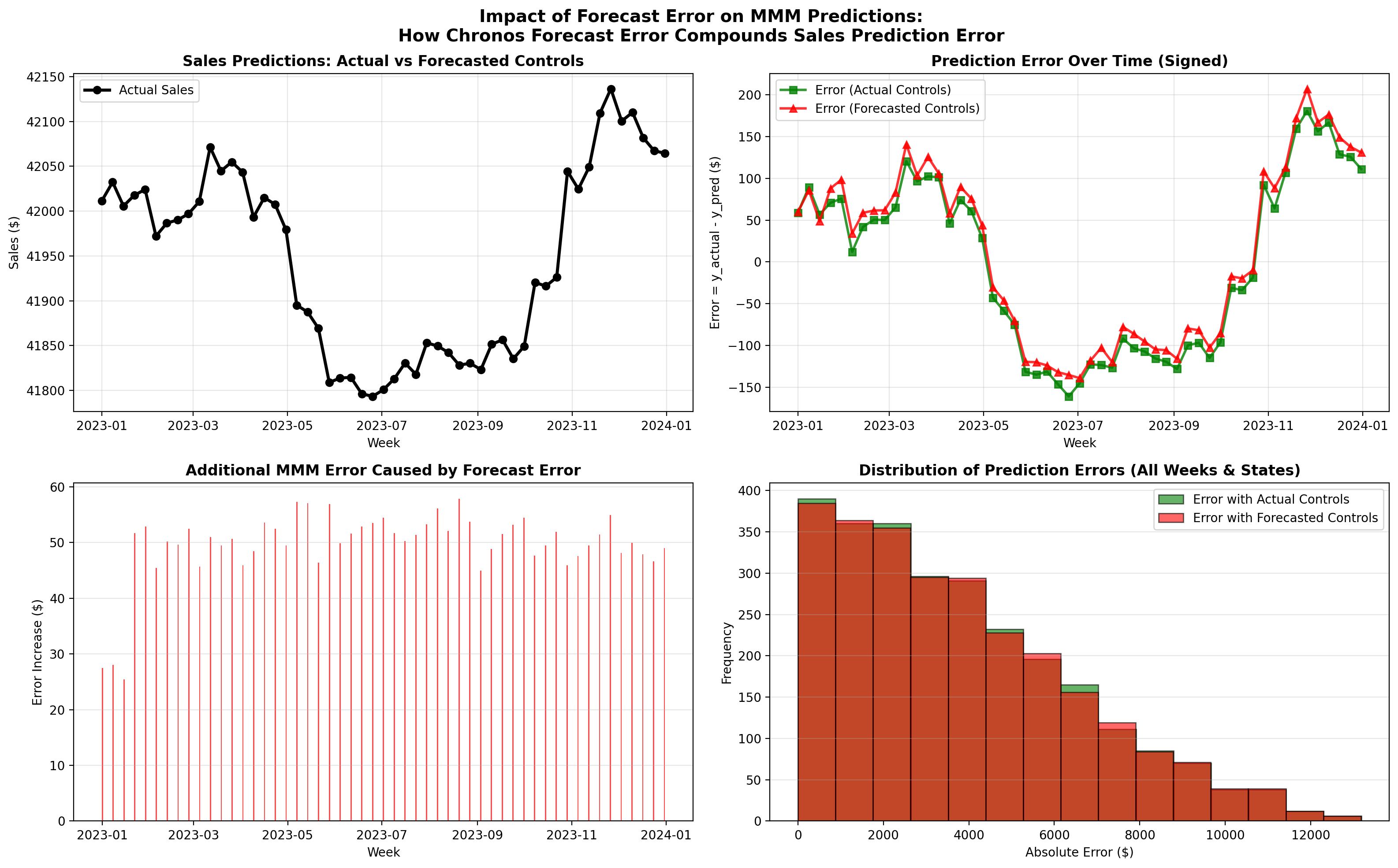
Key Findings:

  • Average additional error from forecast: $49.59

  • Maximum additional error: $1,299.48

  • % of predictions worse with forecasted controls: 50.3%

  • MAPE degradation: +0.03%

  • RMSE degradation: $+15.47

Interpreting the Results

The results above demonstrate the error propagation we discussed in the theory section. Recall the rule of thumb:

Incremental MMM MAPE ≈ Control Share × Control MAPE

Worked Example with Our Data

Using the metrics from this experiment:

1. Control MAPE (from Chronos-2 forecasts): Check the forecast accuracy table above

2. Control Share: Estimated from the MMM coefficients and control values

3. Observed MAPE Degradation: The difference between “With Forecasted Controls” and “With Actual Controls”

The observed degradation should be consistent with the theoretical prediction. If it’s significantly higher, this may indicate:

• Non-linear interactions between controls and media effects

• Model misspecification

• Unusual patterns in the test period

If it’s lower, the model may be robust to control forecast errors, or the controls have limited influence on predictions.

Practical Tips Summary

This section consolidates the key practical recommendations from this tutorial.

When to Use This Approach

This two-model approach (MMM + foundational forecasting model) is appropriate when:

• Your MMM includes control variables that are unavailable for future periods

• The control variables exhibit predictable temporal patterns (seasonality, trends)

• You need forward-looking predictions for budget planning or scenario analysis

Consider simpler alternatives when:

• Controls have minimal influence on predictions (control share < 10%)

• You only need short-term forecasts where last-known values suffice

• Control variables are highly volatile and unpredictable

Key Parameters to Tune

Component	Parameter	Recommendation
MMM	draws, chains	1000+ draws, 4 chains for production
MMM	l_max (adstock)	Match expected carryover duration
Chronos-2	prediction_length	Match your planning horizon
Chronos-2	device	Use “cuda” if GPU available

Expected Accuracy Trade-offs

Use the rule of thumb to set expectations:

\[ \text{Incremental MAPE} \approx \text{Control Share} \times \text{Control MAPE} \]

For example:

• 20% control share × 5% control MAPE = ~1% additional MAPE (acceptable)

• 40% control share × 15% control MAPE = ~6% additional MAPE (may need improvement)

Common Pitfalls and Solutions

Pitfall	Solution
High control forecast error	Try different forecasting models, reduce horizon, or use external forecasts
MMM convergence issues	Increase tuning iterations, adjust priors, check data quality
Inconsistent results across runs	Increase draws and chains, check for multimodality
Memory issues with Chronos-2	Batch forecasts, reduce model size, use CPU if GPU memory limited

Scaling Considerations

For large-scale applications:

• Many geographic units: The multi-dimensional MMM scales well; Chronos-2 can batch forecasts

• Long forecast horizons: Accuracy degrades with horizon; consider rolling forecasts

• Real-time updates: Pre-train MMM, update control forecasts as new data arrives

Conclusion

This tutorial demonstrated how to integrate foundational time series models with PyMC-Marketing MMM to handle the practical challenge of missing control variables in forward-looking predictions.

Key Takeaways

1. The problem is common: Control variables (economic indicators, weather, etc.) are often unavailable for future periods, yet they’re essential for accurate MMM predictions.

2. The solution is modular: By combining a causal model (MMM) with a predictive model (Chronos-2), we leverage the strengths of each—causal understanding from MMM and forecasting accuracy from Chronos-2.

3. Error propagation is predictable: The rule of thumb (Incremental MAPE ≈ Control Share × Control MAPE) provides a practical way to estimate the cost of using forecasted controls.

4. The approach is flexible: While we used Chronos-2, the same framework applies to any forecasting method—ARIMA, Prophet, or domain-specific models.

Limitations

• Assumes linear control effects: The error propagation analysis assumes controls enter the model linearly. Non-linear interactions may cause different behavior.

• Requires forecastable controls: This approach works best when control variables have predictable patterns. Highly volatile or event-driven controls may not forecast well.

• Computational cost: Running both an MMM and a forecasting model adds complexity and compute time.

Next Steps

For practitioners looking to extend this work:

• Experiment with different forecasting models for controls (e.g., Nixtla Models, LightGBM, domain-specific models)

• Incorporate uncertainty from control forecasts into MMM predictions

• Validate the error propagation rule on your specific data

• Consider ensemble approaches that combine multiple control forecasts

References

• Chronos-2: From Univariate to Universal Forecasting - Ansari et al. (2025)

• PyMC-Marketing Documentation

• PyMC-Marketing GitHub Repository

• Amazon Chronos GitHub Repository

%load_ext watermark
%watermark -n -u -v -iv -w

Last updated: Tue, 20 Jan 2026

Python implementation: CPython
Python version       : 3.12.12
IPython version      : 9.6.0

chronos       : 2.0.0
matplotlib    : 3.10.7
numpy         : 2.3.4
pandas        : 2.3.3
polars        : 1.34.0
pymc_marketing: 0.16.0
rich          : 14.2.0
torch         : 2.9.0

Watermark: 2.6.0